How To Remove Minus Values In Excel
Select the columnRow that your X axis numbers are coming from. Select Format Cells Select Number Under the box that has variations of negative numbers select the one that is red without the negative sign.

How To Remove Negative Sign From Numbers In Excel
Click the Data tab and click on the Filter icon.
How to remove minus values in excel. To subtract the numbers in column B from the numbers in column A execute the following steps. Select the cells you want to remove signs and click Kutools Text Remove Characters. Then press Enter key to get the result see screenshot.
How to sum average ignore negative values in Excel. After installing Kutools for Excel please do as follows. Start by right-clicking a cell or range of selected cells and then clicking the.
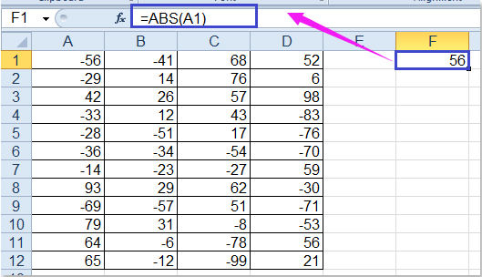
Raw data for excel practice download. To do this type ABS A1 into cell A7. There is an alternative solution to remove characters from the left side using the RIGHT and LEN functions.
Right click and choose Format Cells from the context menu see screenshot. Select the data range that you want to remove the negative signs. To subtract 2 columns row-by-row write a minus formula for the topmost cell and then drag the fill handle or double-click the plus sign to copy the formula to the entire column.
This provides you with the ultimate control over how the data is displayed. Right-click on any of the selected cells and click on Delete Row In the dialog box that opens click on OK. Remove characters from left side using RIGHT and LEN.
At this point you will see no records in the dataset. To average ignore the negative values please use this formula. After free installing Kutools for Excel please do as below.
Simply use the SUM function to shorten your formula. Because of the way Excel handles percentages it sees these formulas as exactly the same thing. F6 has the formula SUM D6E6.
As an example lets subtract numbers in column C from the numbers in column B beginning with row 2. Create a Custom Negative Number Format. If you need to match the negative and positive numbers from the same column that are the same amount eg.
You can also create your own number formats in Excel. In a third cell use the SUM function to add the two cells together. And both of.
Select the range of cells that you want to hide the negative values. This will open the Find and Replace dialog box. In other words It will remove the minus sign if the value is negative and do nothing if the value is positive.
100 -100 then I would use the following formula in the next column. Select the cells that you want to remove leading minus signs and then click Kutools Contents Change Sign of. Enter this formula into a blank cell where you want to put the result SUMIF A1D90 see screenshot.
Thats a quick fix. Select the dataset from which you want to remove the dashes Hold the Control key and then press the H key. IF COUNTIF A1A21A1-1Delete This assumes that the numbers you are comparing are in column A.
In this example cell D6 has the budgeted amount and cell E6 has the actual amount as a negative number. Click Kutools Content Change Sign of Values see screenshot. In the Change Sign of Values dialog box select Change all negative values to positive option see.
Let us follow these steps. SUBSTITUTE A5CHAR CODE LEFT A5 Explanation. This function will return the absolute value of a number.
If there is some other way Id have to play around and research it. The first way to remove a negative sign is by using the ABS function. Type a positive value in one cell and a negative value in another.
Take a look at the screenshot below. For example the formula below subtracts the values in the range A2A9 from the value in cell A1. Remove characters from left side of cell.
An alternative but more long-winded calculation would be to calculate 10 of the number and then subtract it from the original number with one of these formulas. Remove both plus sign and minus sign of each cell with Kutools for Excel. In the Find what field type the dash symbol -.
In the Change Sign of Values dialog check Change all negative values to positive option see screenshot. Then in the Remove Characters dialog check Custom option and type - into the textbox. LEFT A5 grabs the single space code in the formula using LEFT CODE function and giving as input to char function to replace it with an empty string.

Pivot Table To Create List Of Unique Items Remove Duplicates Excel Computer Help Pivot Table

Remove Negative Sign In Excel Excel Tutorials

How To Remove Negative Sign From Numbers In Excel

Use Excel As Your Calculator Excel Workbook Microsoft Excel

Free Excel Inventory Tracking Template Xls Excel Xls Templates Excel Templates Project Management Templates Inventory Management Templates
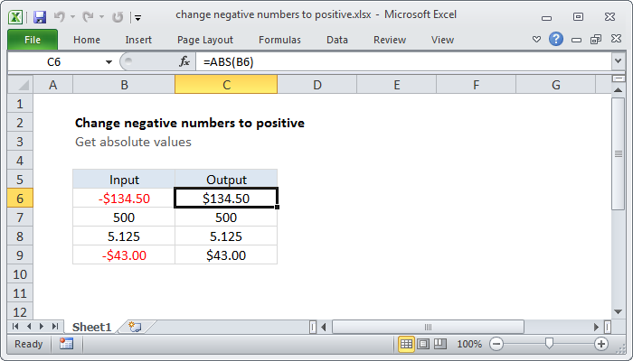
Excel Formula Change Negative Numbers To Positive Exceljet

Abs Tutorial Absolute Value Hindi Remove Any Negative Or Positive Symbols From Numbers Www Myelesson Org Excel Positive Symbols Online Tutorials

How To Remove Negative Sign From Numbers In Excel

Replace Negative Values With Zero In Excel Google Sheets Automate Excel

Excel Formula To Calculate Hours Worked Minus Lunch Excel Formula Excel Shortcuts Excel

How To Remove Negative Sign From Numbers In Excel
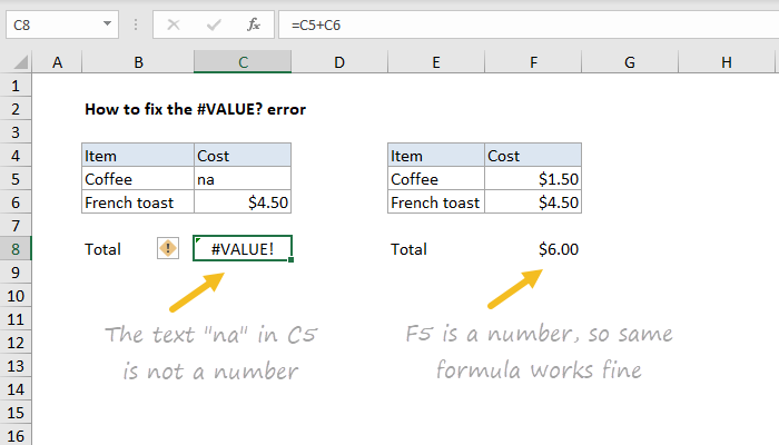
Excel Formula How To Fix The Value Error Exceljet

How To Remove Negative Sign From Numbers In Excel

How To Remove Leading Minus Sign From Numbers In Excel
How To Remove Negative Sign From Numbers In Excel

How To Remove Zeros From Blank Linked Cells How To Remove Cell Computer Programming
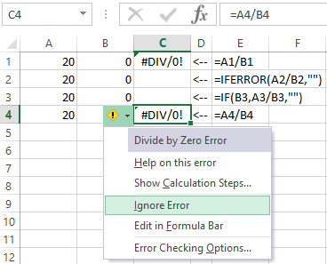
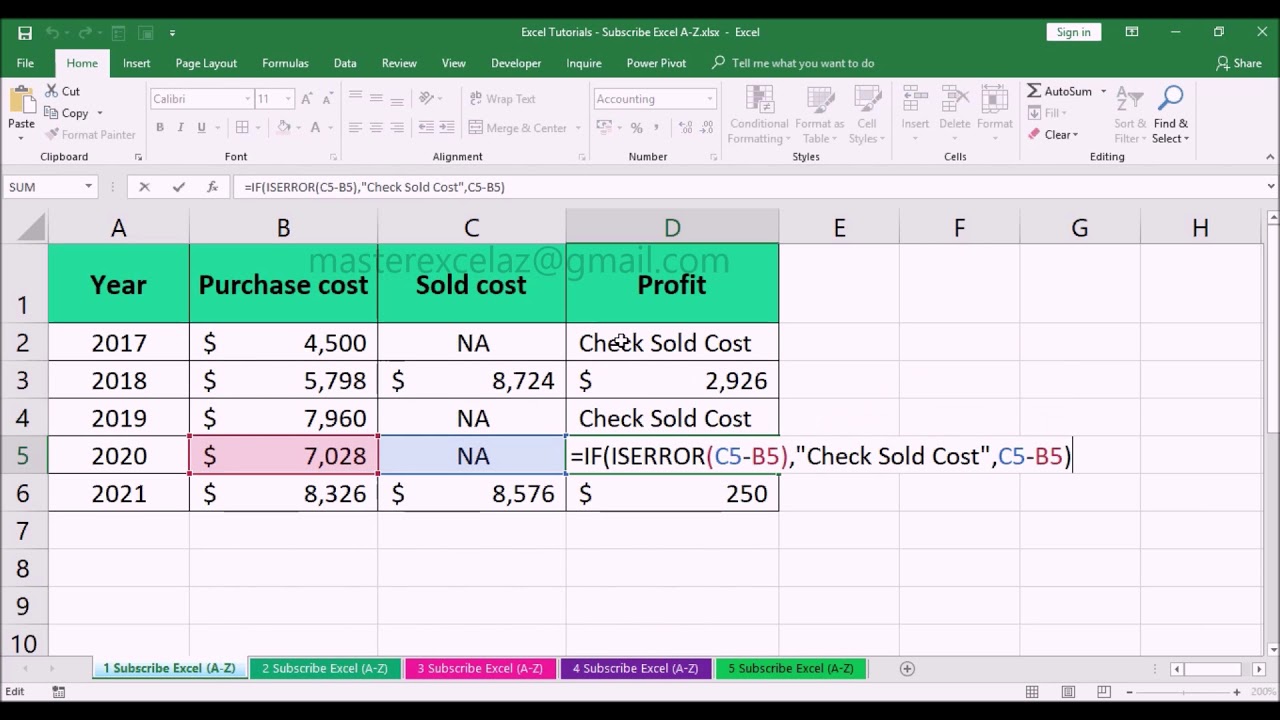
How To Remove Errors In Excel Cells With Formulas

Extract Text Characters With Excel S Left And Leftb Function Excel Function Text
Value Error How To Fix Correct Remove In Ms Excel Spreadsheet 2016 Youtube